好坏质检二分类MLP 实战
任务
1、基于 data-mlp-01.csv 数据,建立 mlp 模型,计算其在测试数据上的准确率,可视化模型预测结果;
2、进行数据分离:test_size=0.33,random_state=10
3、模型结构:一层隐藏层,有 20 个神经元
参考资料
多层感知器MLP(原理)
多层感知器MLP实现非线性分类(原理)
视频:
36.40 实战准备_哔哩哔哩_bilibili
37.41 实战(一)_哔哩哔哩_bilibili
数据准备
数据集名称:data-mlp-01.csv
点我转到百度网盘获取数据集 提取码: 8497
1、原数据可视化
加载数据
#load data
import pandas as pd
import numpy as np
data = pd.read_csv('data-mlp-01.csv')
data.head()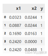
定义 X,y
#define the X and y
X = data.drop(['y'], axis = 1)
y = data.loc[:,'y']
X.head()
可视化
#visualize the data
%matplotlib inline
from matplotlib import pyplot as plt
fig1 = plt.figure(figsize = (5,5))
passed = plt.scatter(X.loc[:,'x1'][y==1], X.loc[:,'x2'][y==1])
failed = plt.scatter(X.loc[:,'x1'][y==0], X.loc[:,'x2'][y==0])
plt.legend((passed, failed),('passed','failed'))
plt.xlabel('x1')
plt.ylabel('x2')
plt.title('raw data')
plt.show()
#蓝色是 y==1 的结果, 橙色的是 y == 0  的结果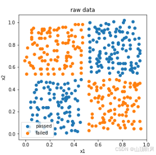
2、数据分离
#split the data
from sklearn.model_selection import train_test_split
X_train, X_test, y_train, y_test = train_test_split(X,y, test_size = 0.33, random_state = 10)
print(X_train.shape, X_test.shape, X.shape)#(275, 2) (136, 2) (411, 2)
3、建立 MLP 模型、训练、预测、可视化
创建模型
# set up the model
from tensorflow.keras.models import Sequential
from tensorflow.keras.layers import Dense, Activationmlp = Sequential()#20:隐藏层神经元个数,input_dim =2 为输入有  x1, x2 两个维度,activation 为激活函数
mlp.add(Dense(units = 20, input_dim = 2, activation = 'sigmoid')) #增加一层输出层,输出层是 1 个神经元,激活函数也是 sigmoid
mlp.add(Dense(units =1, activation = 'sigmoid'))
mlp.summary()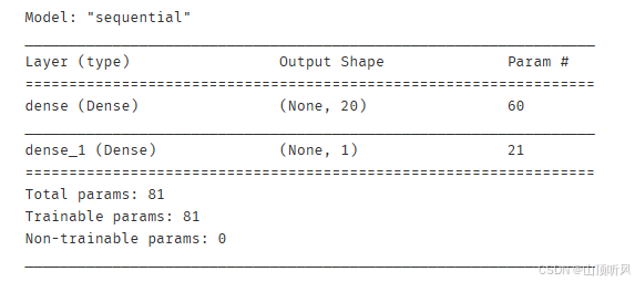
模型配置
#compile the model(模型的配置)
mlp.compile(optimizer = 'adam', loss = 'binary_crossentropy')
# optimizer 为优化方法 ,loss这里用的是 二分类的损失函数
模型训练
#模型的训练
# train the model
mlp.fit(X_train, y_train, epochs = 3000) # epochs 迭代次数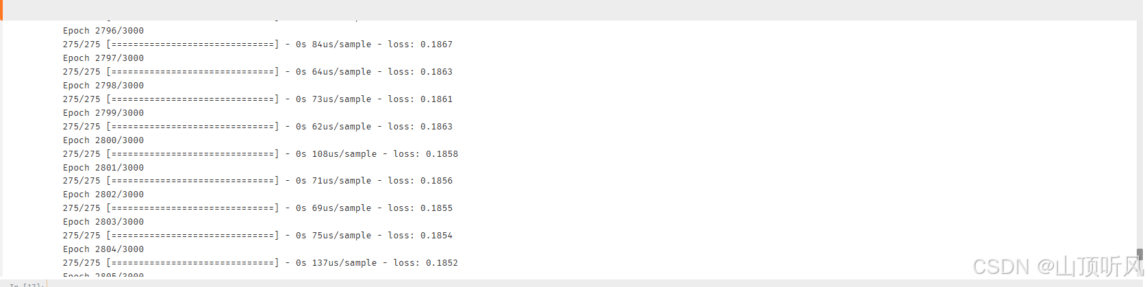
进行预测、计算准确率
训练集
# make prediction and calculate the accuracy
y_train_predict = mlp.predict_classes(X_train)
from sklearn.metrics import accuracy_score
#训练数据集的准确率
accuracy_train = accuracy_score(y_train, y_train_predict)
print(accuracy_train)#0.96
测试集
# 接下来看测试数据集的准确率
y_test_predict = mlp.predict_classes(X_test)
#测试数据集的准确率
accuracy_test = accuracy_score(y_test, y_test_predict)
print(accuracy_test)#0.9632352941176471
#可视化模型的预测结果
#首先看一下输出数据的结构,不合适时进行转换
print(type(y_train_predict)) # <class 'numpy.ndarray'>,不能直接进行索引
y_train_predict_converted = pd.Series(i[0] for i in y_train_predict)
print(y_train_predict_converted)
创建新的数据、进行预测
#创建数据点集
xx,yy = np.meshgrid(np.arange(0,1,0.01), np.arange(0,1,0.01)) # 生成数据,0-1之间,间隔为 0.01
x_range = np.c_[xx.ravel(), yy.ravel()]
#接下来直接进行预测
y_range_predict = mlp.predict_classes(x_range)
print(type(y_range_predict))#<class 'numpy.ndarray'>
#format the output
y_range_predict_converted = pd.Series(i[0] for i in y_range_predict)
print(type(y_range_predict_converted))#<class 'pandas.core.series.Series'>结果可视化
#最后一步,画图,把原来数据点的图拿过来,再加上新的数据点
fig2 = plt.figure(figsize = (5,5))#下面是新创建的数据点(预测数据)
passed_predict = plt.scatter(x_range[:,0][y_range_predict_converted==1],x_range[:,1][y_range_predict_converted==1])
failed_predict = plt.scatter(x_range[:,0][y_range_predict_converted==0],x_range[:,1][y_range_predict_converted==0])
#下面是原来的数据点
passed = plt.scatter(X.loc[:,'x1'][y==1], X.loc[:,'x2'][y==1])
failed = plt.scatter(X.loc[:,'x1'][y==0], X.loc[:,'x2'][y==0])plt.legend((passed, failed, passed_predict, failed_predict),('passed','failed','passed_predict','failed_predict'))
plt.xlabel('x1')
plt.ylabel('x2')
plt.title('prediction result')
plt.show()
#蓝色是 y==1 的结果, 橙色的是 y == 0  的结果
4、好坏质检二分类 mlp 实战 总结
1、通过 mlp 模型,在不增加特征项的情况下,实现了非线性二分类任务;
2、掌握了 mlp 模型的建立、配置与训练方法,并实现基于新数据的预测;
3、熟悉了 mlp 分类的预测数据格式,并实现格式转换;
4、核心算法参考链接:https://keras-cn.readthedocs.io/en/latest/#30skeras